Acoustic wave equation

In physics, the acoustic wave equation is a second-order partial differential equation that governs the propagation of acoustic waves through a material medium resp. a standing wavefield. The equation describes the evolution of acoustic pressure p or particle velocity u as a function of position x and time t. A simplified (scalar) form of the equation describes acoustic waves in only one spatial dimension, while a more general form describes waves in three dimensions.

For lossy media, more intricate models need to be applied in order to take into account frequency-dependent attenuation and phase speed. Such models include acoustic wave equations that incorporate fractional derivative terms, see also the acoustic attenuation article or the survey paper.

Definition in one dimension

The wave equation describing a standing wave field in one dimension (position ${\displaystyle x}$) is

$${\displaystyle p_{xx}-{\frac {1}{c^{2}}}p_{tt}=0,}$$

where ${\displaystyle p}$ is the acoustic pressure (the local deviation from the ambient pressure) and ${\displaystyle c}$ the speed of sound, using subscript notation for the partial derivatives.

Derivation

Start with the ideal gas law

${\displaystyle P=\rho R_{\text{specific}}T,}$

where ${\displaystyle T}$ the absolute temperature of the gas and specific gas constant ${\displaystyle R_{\text{specific}}}$. Then, assuming the process is adiabatic, pressure ${\displaystyle P(\rho )}$ can be considered a function of density ${\displaystyle \rho }$.

The conservation of mass and conservation of momentum can be written as a closed system of two equations $${\displaystyle {\begin{aligned}\rho _{t} (\rho u)_{x}&=0,\\(\rho u)_{t} (\rho u^{2} P(\rho ))_{x}&=0.\end{aligned}}}$$ This coupled system of two nonlinear conservation laws can be written in vector form as: $${\displaystyle q_{t} f(q)_{x}=0,}$$ with $${\displaystyle q={\begin{bmatrix}\rho \\\rho u\end{bmatrix}}={\begin{bmatrix}q_{(1)}\\q_{(2)}\end{bmatrix}},\quad f(q)={\begin{bmatrix}\rho u\\\rho u^{2} P(\rho )\end{bmatrix}}={\begin{bmatrix}q_{(2)}\\q_{(2)}^{2}/q_{(1)} P(q_{(1)})\end{bmatrix}}.}$$

To linearize this equation, let $${\displaystyle q(x,t)=q_{0} {\tilde {q}}(x,t),}$$ where ${\displaystyle q_{0}=(\rho _{0},\rho _{0}u_{0})}$ is the (constant) background state and ${\displaystyle {\tilde {q}}}$ is a sufficiently small perturbation, i.e., any powers or products of ${\displaystyle {\tilde {q}}}$ can be discarded. Hence, the taylor expansion of ${\displaystyle f(q)}$ gives: $${\displaystyle f(q_{0} {\tilde {q}})\approx f(q_{0}) f'(q_{0}){\tilde {q}}}$$ where $${\displaystyle f'(q)={\begin{bmatrix}\partial f_{(1)}/\partial q_{(1)}&\partial f_{(1)}/\partial q_{(2)}\\\partial f_{(2)}/\partial q_{(1)}&\partial f_{(2)}/\partial q_{(2)}\end{bmatrix}}={\begin{bmatrix}0&1\\-u^{2} P'(\rho )&2u\end{bmatrix}}.}$$ This results in the linearized equation $${\displaystyle {\tilde {q}}_{t} f'(q_{0}){\tilde {q}}_{x}=0\quad \Leftrightarrow \quad {\begin{aligned}{\tilde {\rho }}_{t} ({\widetilde {\rho u}})_{x}&=0\\({\widetilde {\rho u}})_{t} (-u_{0}^{2} P'(\rho _{0})){\tilde {\rho }}_{x} 2u_{0}({\widetilde {\rho u}})_{x}&=0\end{aligned}}}$$ Likewise, small perturbations of the components of ${\displaystyle q}$ can be rewritten as: $${\displaystyle \rho u=(\rho _{0} {\tilde {\rho }})(u_{0} {\tilde {u}})=\rho _{0}u_{0} {\tilde {\rho }}u_{0} \rho _{0}{\tilde {u}} {\tilde {\rho }}{\tilde {u}}}$$ such that $${\displaystyle {\widetilde {\rho u}}\approx {\tilde {\rho }}u_{0} \rho _{0}{\tilde {u}},}$$ and pressure perturbations relate to density perturbations as: $${\displaystyle p=p_{0} {\tilde {p}}=P(\rho _{0} {\tilde {\rho }})=P(\rho _{0}) P'(\rho _{0}){\tilde {\rho }} \dots }$$ such that: $${\displaystyle p_{0}=P(\rho _{0}),\quad {\tilde {p}}\approx P'(\rho _{0}){\tilde {\rho }},}$$ where ${\displaystyle P'(\rho _{0})}$ is a constant, resulting in the alternative form of the linear acoustics equations: $${\displaystyle {\begin{aligned}{\tilde {p}}_{t} u_{0}{\tilde {p}}_{x} K_{0}{\tilde {u}}_{x}&=0,\\\rho _{0}{\tilde {u}}_{t} {\tilde {p}}_{x} \rho _{0}u_{0}{\tilde {u}}_{x}&=0.\end{aligned}}}$$ where ${\displaystyle K_{0}=\rho _{0}P'(\rho _{0})}$ is the bulk modulus of compressibility. After dropping the tilde for convenience, the linear first order system can be written as: $${\displaystyle {\begin{bmatrix}p\\u\end{bmatrix}}_{t} {\begin{bmatrix}u_{0}&K_{0}\\1/\rho _{0}&u_{0}\end{bmatrix}}{\begin{bmatrix}p\\u\end{bmatrix}}_{x}=0.}$$ While, in general, a non-zero background velocity is possible (e.g. when studying the sound propagation in a constant-strength wind), it will be assumed that ${\displaystyle u_{0}=0}$. Then the linear system reduces to the second-order wave equation: $${\displaystyle p_{tt}=-K_{0}u_{xt}=-K_{0}u_{tx}=K_{0}\left({\frac {1}{\rho _{0}}}p_{x}\right)_{x}=c_{0}^{2}p_{xx},}$$ with ${\displaystyle c_{0}={\sqrt {K_{0}/\rho _{0}}}}$ the speed of sound.

Hence, the acoustic equation can be derived from a system of first-order advection equations that follow directly from physics, i.e., the first integrals: $${\displaystyle q_{t} Aq_{x}=0,}$$ with $${\displaystyle q={\begin{bmatrix}p\\u\end{bmatrix}},\quad A={\begin{bmatrix}0&K_{0}\\1/\rho _{0}&0\end{bmatrix}}.}$$ Conversely, given the second-order equation ${\displaystyle p_{tt}=c_{0}^{2}p_{xx}}$ a first-order system can be derived: $${\displaystyle q_{t} {\hat {A}}q_{x}=0,}$$ with $${\displaystyle q={\begin{bmatrix}p_{t}\\-p_{x}\end{bmatrix}},\quad {\hat {A}}={\begin{bmatrix}0&c_{0}^{2}\\1&0\end{bmatrix}},}$$ where matrix ${\displaystyle A}$ and ${\displaystyle {\hat {A}}}$ are similar.

Solution

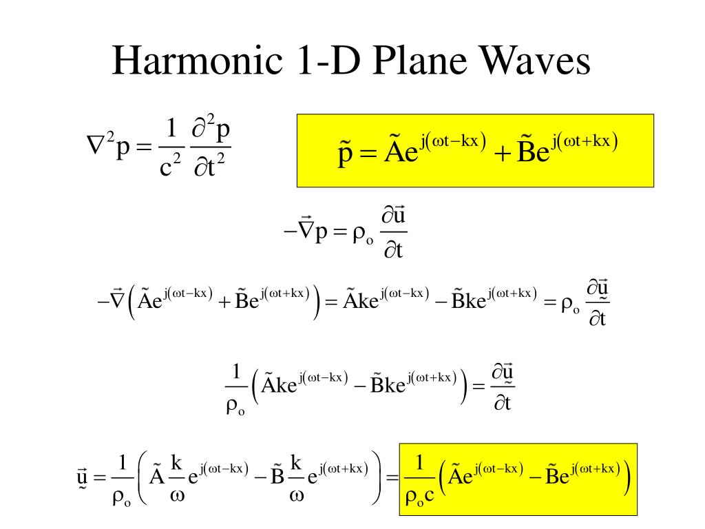
Provided that the speed ${\displaystyle c}$ is a constant, not dependent on frequency (the dispersionless case), then the most general solution is

${\displaystyle p=f(ct-x) g(ct x)}$

where ${\displaystyle f}$ and ${\displaystyle g}$ are any two twice-differentiable functions. This may be pictured as the superposition of two waveforms of arbitrary profile, one (${\displaystyle f}$) traveling up the x-axis and the other (${\displaystyle g}$) down the x-axis at the speed ${\displaystyle c}$. The particular case of a sinusoidal wave traveling in one direction is obtained by choosing either ${\displaystyle f}$ or ${\displaystyle g}$ to be a sinusoid, and the other to be zero, giving

${\displaystyle p=p_{0}\sin(\omega t\mp kx)}$.

where ${\displaystyle \omega }$ is the angular frequency of the wave and ${\displaystyle k}$ is its wave number.

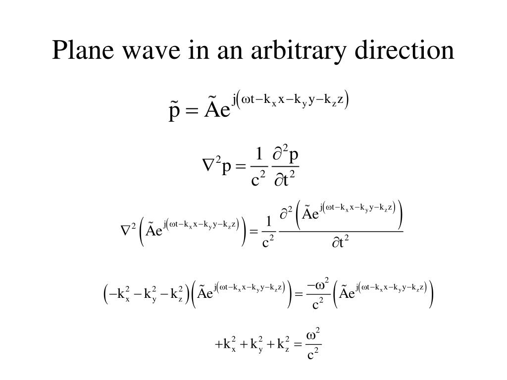
In three dimensions

Equation

Feynman provides a derivation of the wave equation for sound in three dimensions as

${\displaystyle \nabla ^{2}p-{1 \over c^{2}}{\partial ^{2}p \over \partial t^{2}}=0,}$

where ${\displaystyle \nabla ^{2}}$ is the Laplace operator, ${\displaystyle p}$ is the acoustic pressure (the local deviation from the ambient pressure), and ${\displaystyle c}$ is the speed of sound.

A similar looking wave equation but for the vector field particle velocity is given by

${\displaystyle \nabla ^{2}\mathbf {u} \;-{1 \over c^{2}}{\partial ^{2}\mathbf {u} \; \over \partial t^{2}}=0}$.

In some situations, it is more convenient to solve the wave equation for an abstract scalar field velocity potential which has the form

${\displaystyle \nabla ^{2}\Phi -{1 \over c^{2}}{\partial ^{2}\Phi \over \partial t^{2}}=0}$

and then derive the physical quantities particle velocity and acoustic pressure by the equations (or definition, in the case of particle velocity):

${\displaystyle \mathbf {u} =\nabla \Phi \;}$,

${\displaystyle p=-\rho {\partial \over \partial t}\Phi }$.

Solution

The following solutions are obtained by separation of variables in different coordinate systems. They are phasor solutions, that is they have an implicit time-dependence factor of ${\displaystyle e^{i\omega t}}$ where ${\displaystyle \omega =2\pi f}$ is the angular frequency. The explicit time dependence is given by

${\displaystyle p(r,t,k)=\operatorname {Real} \left[p(r,k)e^{i\omega t}\right]}$

Here ${\displaystyle k=\omega /c\ }$ is the wave number.

Cartesian coordinates

${\displaystyle p(r,k)=Ae^{\pm ikr}}$.

Cylindrical coordinates

${\displaystyle p(r,k)=AH_{0}^{(1)}(kr) \ BH_{0}^{(2)}(kr)}$.

where the asymptotic approximations to the Hankel functions, when ${\displaystyle kr\rightarrow \infty }$, are

${\displaystyle H_{0}^{(1)}(kr)\simeq {\sqrt {\frac {2}{\pi kr}}}e^{i(kr-\pi /4)}}$

${\displaystyle H_{0}^{(2)}(kr)\simeq {\sqrt {\frac {2}{\pi kr}}}e^{-i(kr-\pi /4)}}$.

Spherical coordinates

${\displaystyle p(r,k)={\frac {A}{r}}e^{\pm ikr}}$.

Depending on the chosen Fourier convention, one of these represents an outward travelling wave and the other a nonphysical inward travelling wave. The inward travelling solution wave is only nonphysical because of the singularity that occurs at r=0; inward travelling waves do exist.

See also

• Acoustics
• Acoustic attenuation
• Acoustic theory
• Differential equations
• Fluid dynamics
• Ideal gas law
• Madelung equations
• One-way wave equation
• Pressure
• Thermodynamics
• Wave equation

Notes

References

• LeVeque, Randall J. (2002). Finite Volume Methods for Hyperbolic Problems. Cambridge University Press. doi:10.1017/cbo9780511791253. ISBN 978-0-521-81087-6.